Today marks a major moment in the development of a project I’ve been working on for some time: me and my co-authors have completed a paper on inferring the opening angles of gamma ray bursts by observing binary neutron star mergers and gamma ray bursts. What does that mean? Well, I guess the point of this post is to explain just that. It should be said, while you can download the paper now, it’s still a pre-print: that means it hasn’t been peer-reviewed yet, so there’s a chance it may contain some mistakes which we’ve not picked up on. So I guess you might argue it’s probably not quite completed.
Gamma ray bursts (GRBs) are the brightest things which we ever observe in the electromagnetic spectrum (which includes all of the radiation we encounter in day-to-day life, like light, radio-waves, microwaves, and x-rays). GRBs produce most of their emission in the most energetic part of that spectrum - what we call “gamma rays”. We don’t encounter this type of radiation very frequently in normal life, which is just as well, as even in quite small doses it can be quite bad for you - it is, however, produced by some types of radioactive decay.
Until recently we weren’t completely sure what caused these bursts, but astronomers suspected that some of them, a group called “short GRBs” were probably the result of two neutron stars (the neutron-rich corpses of dead stars) crashing into each other - an event which is known as a binary neutron star merger (or BNS for short). These BNS events are notable for something else - until recently they were one of the most likely candidates for being detected by gravitational wave observatories like LIGO, but in August this year they moved from being just a likely source to being a confirmed one, as we observed GW170817, the merger between two neutron stars, using gravitational waves. A (very) short time later two gamma ray observatories detected a gamma ray burst, which confirmed that BNS events were the source of at least some GRBs.
Gamma ray bursts emit their energy in a beam along their rotation axis (which is a result, in part, of how quickly they’re rotating), but we can’t tell just from looking at the burst what shape this beam is. (The GRB associated with GW170817 complicates things even more, because we might not actually have seen it inside its main beam, but that’s another matter). There are some physical arguments you can make to work out limits on how big the beam can be, but it requires making various assumptions.
Our method
We set out to find a way of working out limits on the size of the beam while assuming as little as possible about the underlying physics, which means that we can give more robust (if sometimes less impressive-looking) statements about what’s going on in the GRB. It turns out that you can do that just using geometry and by counting the number of GRBs you see, and the number of BNS events you record using gravitational wave detectors. This is possible because the gravitational wave emission isn’t beamed, and so we expect to see all of the BNS events which happen while our detectors are turned on, which are within the region of space which they’re sensitive to.
Comparing these two numbers directly assumes that all BNS events “launch” a GRB, which is a physical assumption that we decided we didn’t want to make, and so we also include an additional parameter - the efficiency with which a GRB is produced. Our analysis is conducted in a Bayesian framework, which makes it easy to “marginalise over” this parameter at the end, so that our results take it into account.
An intuitive way to think about how doing this works goes a bit like this: say you detect gravitational waves from a BNS, but you don’t see a GRB to go with it. What does that tell you? It tells you that the emission is beamed (so the opening angle isn’t 90-degrees), but you can’t say an awful lot about the shape of the beam from just one observation. However, if after watching for longer, you find that you see one GRB for every ten BNS observations you can start to infer that the beam must be quite small (and so you need to be reasonably “lucky” to be able to see it). Likewise, if you saw nine GRBs to go with your ten BNS events you might conclude that the beam was pretty wide.
Results
In this paper we don’t actually analyse any real data: we’re looking at what can happen in a set of hypothetical scenarios which are believed to be the most likely situations that the LIGO detectors will find themselves in over the next decade.
To that end, we started by looking at what happens when you run your gravitational wave detector for some period of time, and don’t see any BNS events; we chose to use the “scenario” which had been predicted for our first observing run (you can read more about the predictions for how long each observing run will last, and what they’re expected to detect in this paper).
Because we didn’t want to make any firm statement about the efficiency at which GRBs are produced by BNS events, we worked out what the results would look like in all four cases, and those are in the plot in figure 1.
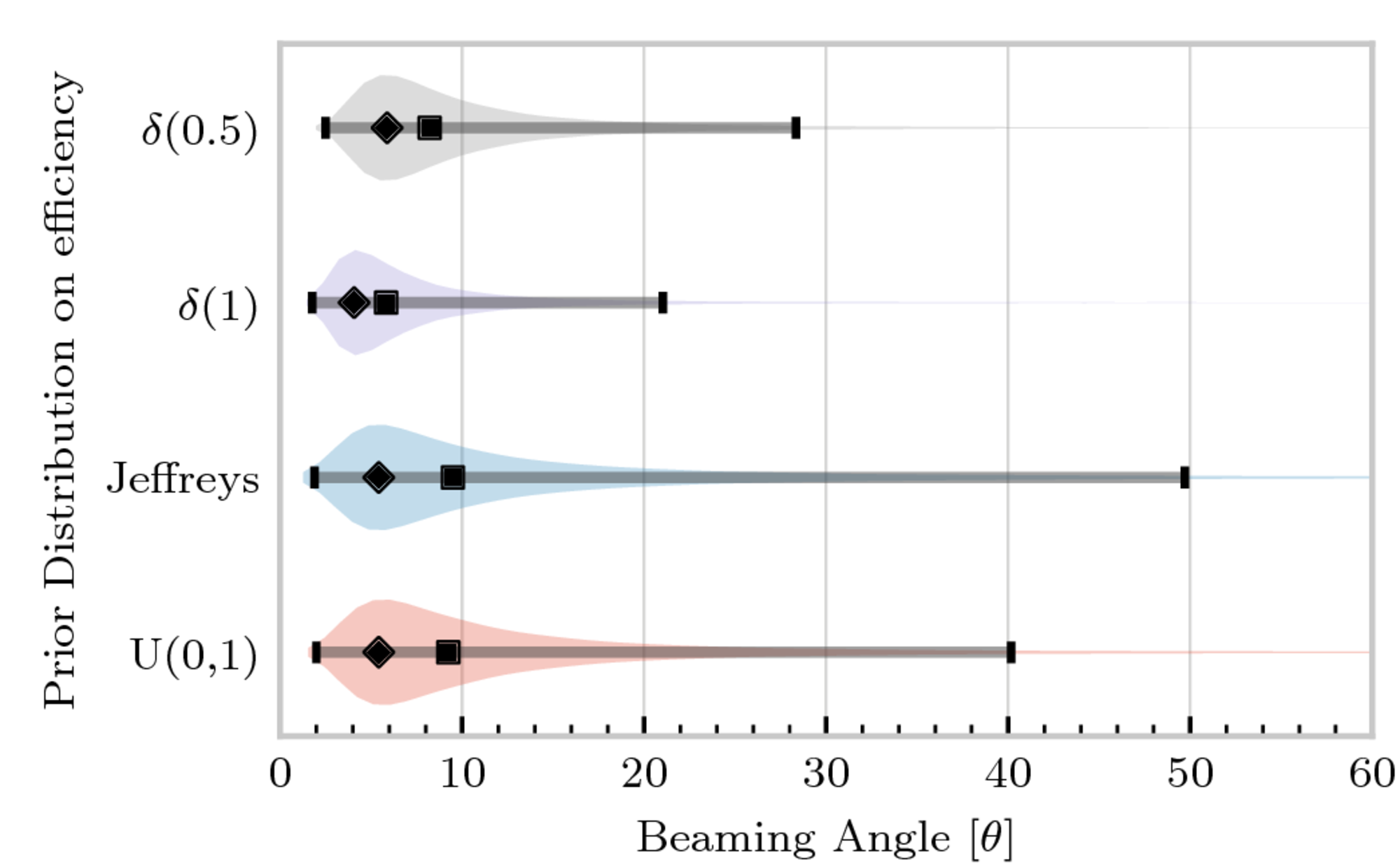
We did this to demonstrate that even when you make no BNS detections, you can make a statement about the beaming angle. The weakest statement about our prior knowledge of the efficiency is made by the Jeffreys prior, which attempts to be uninformative, and so we get a broad range of possible values from it. In contrast, the “delta(1)” prior, which assumes that all BNS events produce a GRB, produces a narrower range. This is the assumption which is normally made about GRB efficiency.
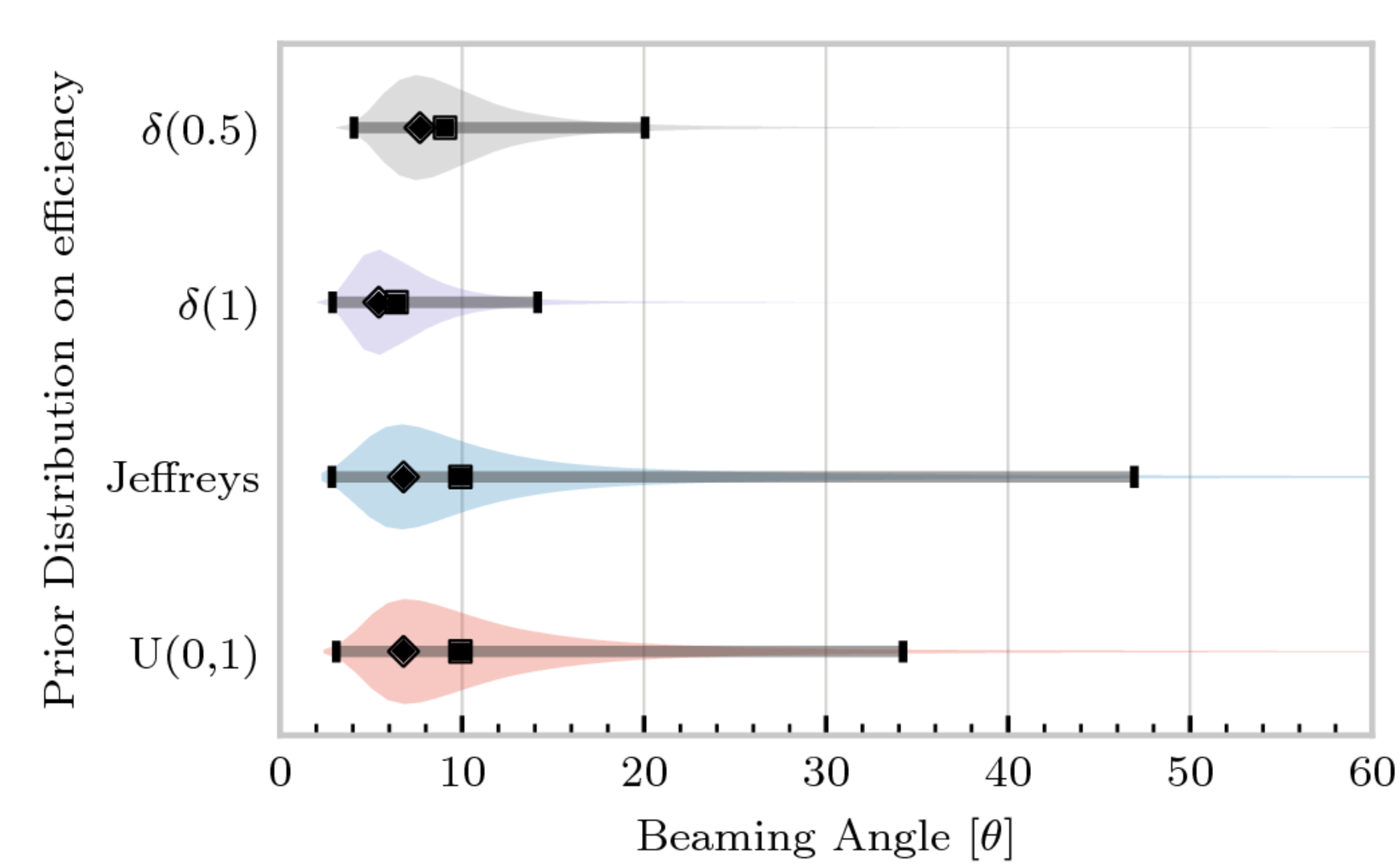
We then turned to the predicted scenario for O2, where we predicted a reasonable probability that one BNS detection would be made (and, as it turned out, one detection was made), and those results are in figure 2.
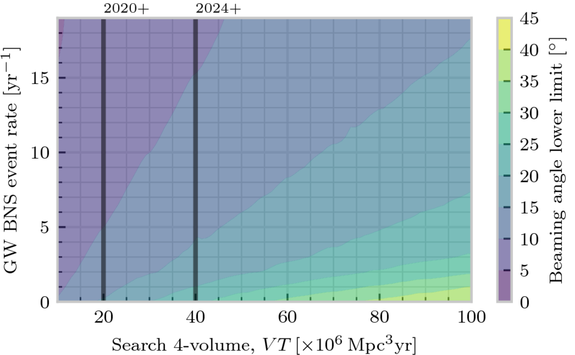
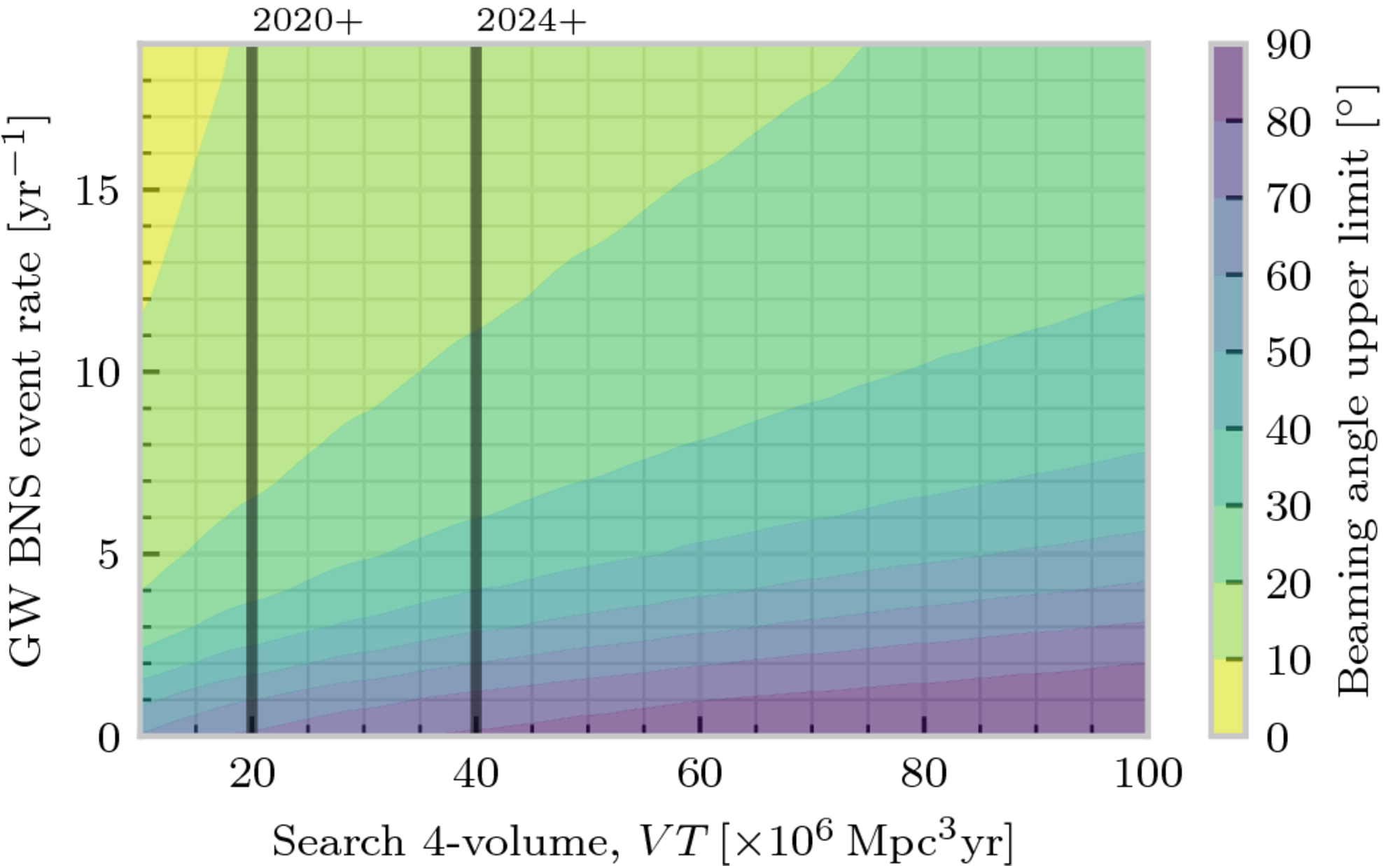
In order to complete our analysis we looked at how a range of observing times and detector sensitivities would affect the analysis, producing the rather colourful plots in figures 3 and 4 which show how the lower limit on our posterior changes (figure 3) along with the upper limit (figure 4) as we both observe for longer and observe more BNSes per year.